Implementing metrics in Go
Metrics are data points representing your system behaviour over time. People instrument their long-running apps with metrics to see if there are or were any problems and if the system behaves as expected.
There are various metric types, but most common ones are counters, gauges and histograms.
Metric types
Counter is simply an increasing number. You may use counters to track the number of served requests, number of errors, and so on. If you are only interested to see how many times a certain event has happened during the given time frame - use a counter.
Counters are probably the simplest metrics and the only information they provide is a single number - counter value.
Gauge is also a number, but it may go up and down. You may use gauges to track the memory usage, CPU load, temperature and other measured values.
Unlike counters, gauges often track not only their current value, but also their mean, minimum and maximum values for each time interval.
However, mean is not always the right characteristic to look at. In practice there are many cases when percentiles are more meaningful that a mean. To track percentiles histogram metrics are used.
For those who are unaware of percentiles - it is a number such that a certain percentage of values fall below that number. Here’s a good explanation when percentiles could be more useful than averages.
The most typical use case is tracking response times. For example, 95th percentile of the response times shows the maximum response time of the 95% of the requests.
Implementation
I like explaining things by showing how they work. All the code below is simplified and the real implementation is slightly different (here we don’t focus on thread safety, division by zero errors etc).
Let’s consider a generic meter. What can it do? It can accept an incoming numerical value, one at a time, or it can be reset back to its zero state.
type Metric interface {
	Add(n float64)
	Reset()
}
There are two approaches to do metircs. One is to record every single event and run queries each time to calculate the metrics. It’s the most precise and flexible approach, although it’s time-consuming and needs more storage. Another is to calculate metric values on the fly. It often uses less memory and is good enough for most use cases, so we will go this way.
Let’s start with the counter, since it is probably the easiest metric to implement:
type Counter float64
func (c *Counter) Add(n float64) { *c = *c + Counter(n) }
func (c *Counter) Reset() { *c = 0 }
Gauge needs to track mean, min and max values. To calculate rolling mean we need to count the number of events and their sum value:
type Gauge struct {
	count int
	sum   float64
	min   float64
	max   float64
}
func (g *Gauge) Reset() { g.count, g.sum, g.min, g.max = 0, 0, 0, 0 }
func (g *Gauge) mean() float64 { return g.sum / g.count }
func (g *Gauge) Add(n float64) {
	if n < g.min { g.min = n }
	if n > g.max { g.max = n }
	g.count++
	g.sum = g.sum + n
}
Finally, histograms. There seems to be no easy way to build precise histograms without remembering all the data entries. However there are some algorithms to construct approximate histograms on the fly.
One such algorithm has a fixed number of bins, puts a new incoming value into an individual bin and when there are too many bins - it merges two most similar ones.
type bin struct {
	value float64
	count float64
}
type Histogram struct {
	bins  []bin
	total uint64
}
func (h *Histogram) Reset() { h.bins, h.total = 0, nil }
func (h *Histogram) Add(n float64) {
	defer h.trim()
	h.total++
	newbin := bin{value: n, count: 1}
	// Insert new bin with a single value into the sorted array of bins
	for i := range h.bins {
		if h.bins[i].value > n {
			h.bins = append(h.bins[:i], append([]bin{newbin}, h.bins[i:]...)...)
			return
		}
	}
	h.bins = append(h.bins, newbin)
}
func (h *Histogram) trim() {
	for len(h.bins) > maxBins {
		// Find two adjacent bins with the closest values
		d := float64(0)
		i := 0
		for j := 1; j < len(h.bins); j++ {
			if delta := h.bins[j].value - h.bins[j-1].value; delta < d || j == 1 {
				d = delta
				i = j
			}
		}
		// Merge bins
		count := h.bins[i-1].count + h.bins[i].count
		merged := bin{
			value: (h.bins[i-1].value*h.bins[i-1].count + h.bins[i].value*h.bins[i].count) / count,
			count: count,
		}
		// Remove the second bin
		h.bins = append(h.bins[:i-1], h.bins[i:]...)
		h.bins[i-1] = merged
	}
}
This approach may not be the most precise, but it shows the overall picture of how your data is distributed.
Timelines and multiple metrics
Once we’ve implemented individual metrics - we can easliy build a timeline. Timeline is a slice of buckets, where each bucket contains metric values for one time slot. Timeline is rotated as time goes.
Also, it is often helpful to store timelines with multiple precisions. E.g. to store one month of data with hourly precision and 6 hours of data with 30 seconds precision.
Since all metrics share a common interface - a combination of metrics can also implement the same interface.
I won’t provide actual implementations here, since they are really trivial.
To construct a metric there will be thee constructor functions: NewCounter,
NewGauge or NewHistogram. If no parameters are given - you will get a
single meter. You may also provide a number of precision strings to get
historical timelines of the given metric type. Precision strings look like
“30m1s” which means “I want a timeline for 30 minutes of historical data with 1
second precision”:
// A meter that keeps gauges for 30 days, 48 hours and 15 minutes of time with
// different precision:
m := metric.NewGauge("30d1h", "48h5m", "15m1s")
...
m.Add(someValue)
expvar and web interface
Now we can construct metrics and push data. Two questions remain: how to access metrics throughout your app code and how to actually read metric data.
Go provides an infamous expvar package to keep “exposed” public variables.
This variables can be read using a builtin HTTP endpoint /debug/metrics as a
JSON. I think it is a good idea not to reinvent the wheel and just integrate
out metrics with expvar. It is done by simply implementing a String()
method that prints metric data as a JSON string.
In addition to that, expvar also provides a simple API to register metric and
to get it, although some type casting is needed:
// Register metrics
expvar.Publish("num_errors", metric.NewCounter("15m10s"))
expvar.Publish("latency", metric.NewHistogram("5m1s", "15m30s", "1h1m"))

// Measure time and update the metric
start := time.Now()
...
expvar.Get("latency").(metric.Metric).Add(time.Since(start).Seconds())

// Update counter
expvar.Get("num_errors").(metric.Metric).Add(1)
I like using standard libraries as much as possible, but I also believe that visual representation of data is better than reading plain JSON. So this metrics package includes an opinionated web UI:
http.Handle("/debug/metrics", metric.Handler(metric.Exposed))
Here’s how it looks like:
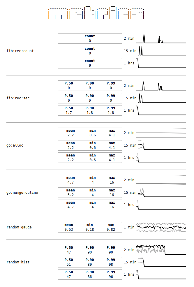
On some graphs there are three lines. Of gauges the black line is the mean, while gray lines are min and max. For histograms the black line is 99th percentile, while gray lines are 90th and 50th percentiles.
The web UI uses no javascript and is very fast even if the number of metrics is high.
Summary
You may find all the source code at https://github.com/zserge/metric. It’s very small, a single file of ~300 lines of code and a few more lines for the user interface. The library has no external dependencies and it’s really featherweight.
If you are building something big and it should scale well - consider using real tools such as Prometheus, InfluxDB or StatsD. But for smaller projects if you want to avoid wasting time to configure all those tools - feel free to use this package, the setup is no harder than just importing a package and you can start tracking you metrics almost immediately.
Of course, if you found an issue or have a suggestion - don’t hesitate to drop me a line or open an issue!
I hope you’ve enjoyed this article. You can follow – and contribute to – on Github, Mastodon, Twitter or subscribe via rss.
Jun 10, 2018
