By the power of grayscale!
When people talk about computer vision, they usually think of OpenCV or deep neural networks like YOLO. But in most cases, doing computer vision implies understanding of the core algorithms, so you can use or adapt them for your own needs.
I wanted to see how far I could go by stripping computer vision down to the bare minimum: only grayscale 8-bit images, no fancy data structures, plain old C, some byte arrays and a single header file. After all, an image is just a rectangle of numbers, right?
This post is a guided tour through the algorithms behind Grayskull – a minimal computer vision library designed for resource-constrained devices.
Pixels
A grayscale pixel is normally represented as a single byte, where 0 means black, 255 means white, and values in between represent various shades of gray.
A grayscale image is essentially a 2D array of these pixels, defined by its width and height, but for a simpler memory layout languages such as C often represent it as a 1D array of size width * height:
// An image of WxH pixels, stored as a flat array of bytes
struct gs_image { unsigned w, h; uint8_t *data; };

// Helpers to get/set pixel values respecting the bounds
uint8_t gs_get(struct gs_image img, unsigned x, unsigned y) {
  return (x < img.w && y < img.h) ? img.data[y * img.w + x] : 0;
}
void gs_set(struct gs_image img, unsigned x, unsigned y, uint8_t value) {
  if (x < img.w && y < img.h) img.data[y * img.w + x] = value;
}

// A somewhat convenient macro to iterate over all pixels
#define gs_for(img, x, y)                \
  for (unsigned y = 0; y < (img).h; y++) \
    for (unsigned x = 0; x < (img).w; x++)
This humble start already allows us to do some tricks like inverting or mirroring images:
// invert image (negative): px[x,y] = 255 - px[x,y]
gs_for(img, x, y) gs_set(img, x, y, 255 - gs_get(img, x, y));

// mirror the image: swap px[x,y] with px[w-x-1,y]
gs_for(img, x, y) {
for (unsigned y = 0; y < img.h; y++) {
  for (unsigned x = 0; x < img.w/2; x++) { // iterate only through the first half
    uint8_t tmp = gs_get(img, x, y);
    gs_set(img, x, y, gs_get(img, img.w - x - 1, y));
    gs_set(img, img.w - x - 1, y, tmp);
  }
}
We can just as well copy images, crop images, resize or rotate them. It’s not computer vision yet, but still some basic image processing:
struct gs_rect { unsigned x, y, w, h; }; // for regions of interest (ROI)

// crop image src into dst using region of interest (roi)
gs_for(roi, x, y) gs_set(dst, x, y, gs_get(src, roi.x + x, roi.y + y));

// downscale 2x: set pixel to average from 4 neighbouring pixels (2x2)
gs_for(dst, x, y) {
    unsigned sum = 0;
    for (unsigned j = 0; j < 2; j++)
      for (unsigned i = 0; i < 2; i++)
        sum += gs_get(src, x * 2 + i, y * 2 + j);
    gs_set(dst, x, y, sum / 4);
}
One can do naïve nearest-neighbour resizing, which is fast but looks blocky, or do bilinear interpolation, which is slower and requires floating point operations, but often looks better:
// Nearest-neighbour resize
void gs_resize_nn(struct gs_image dst, struct gs_image src) {
    gs_for(dst, x, y) {
        unsigned sx = x * src.w / dst.w, sy = y * src.h / dst.h;
        gs_set(dst, x, y, gs_get(src, sx, sy));
    }
}

// Bilinear resize
GS_API void gs_resize(struct gs_image dst, struct gs_image src) {
  gs_for(dst, x, y) {
    float sx = ((float)x + 0.5f) * src.w / dst.w, sy = ((float)y + 0.5f) * src.h / dst.h;
    sx = GS_MAX(0.0f, GS_MIN(sx, src.w - 1.0f)), sy = GS_MAX(0.0f, GS_MIN(sy, src.h - 1.0f));
    unsigned sx_int = (unsigned)sx, sy_int = (unsigned)sy;
    unsigned sx1 = GS_MIN(sx_int + 1, src.w - 1), sy1 = GS_MIN(sy_int + 1, src.h - 1);
    float dx = sx - sx_int, dy = sy - sy_int;
    uint8_t c00 = gs_get(src, sx_int, sy_int), c01 = gs_get(src, sx1, sy_int),
            c10 = gs_get(src, sx_int, sy1), c11 = gs_get(src, sx1, sy1);
    uint8_t p = (c00 * (1 - dx) * (1 - dy)) + (c01 * dx * (1 - dy)) + (c10 * (1 - dx) * dy) + (c11 * dx * dy);
    gs_set(dst, x, y, p);
  }
}
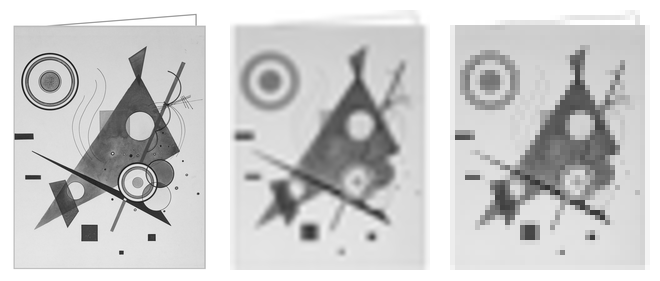
Here’s how the original image (left) looks after bilinear resizing (middle) compared to nearest-neighbour resizing (right).
Image processing
Now that we can manipulate individual pixels, we can start doing more serious image processing.
One useful tool is convolutional filters. A filter is a small 2D array (kernel) that is applied to each pixel in the image. The new pixel value is computed as a weighted sum of the neighbouring pixels, where weights are defined by the kernel.
void gs_filter(struct gs_image dst, struct gs_image src, struct gs_image kernel, unsigned norm) {
    gs_for(dst, x, y) {
        int sum = 0;
        gs_for(kernel, i, j) {
            sum += gs_get(src, x + i - kernel.w / 2, y + j - kernel.h / 2) * (int8_t)gs_get(kernel, i, j);
        }
        gs_set(dst, x, y, sum / norm);
    }
}
This technique can be used for blurring, sharpening, edge detection and many other effects. Here are some common kernels. Note that they are defined as signed 8-bit integers:
// box blur 3x3, all pixels have equal weight
struct gs_image gs_blur_box = {3, 3, (uint8_t *)(int8_t[]){1, 1, 1, 1, 1, 1, 1, 1, 1}};
// gaussian blur 3x3, central pixels have more weight
struct gs_image gs_blur_gaussian = {3, 3, (uint8_t *)(int8_t[]){1, 2, 1, 2, 4, 2, 1, 2, 1}};
// sharpen, enhance edges
struct gs_image gs_sharpen = {3, 3, (uint8_t *)(int8_t[]){0, -1, 0, -1, 5, -1, 0, -1, 0}};
// emboss, make image look "3D"
struct gs_image gs_emboss = {3, 3, (uint8_t *)(int8_t[]){-2, -1, 0, -1, 1, 1, 0, 1, 2}};
Similarly, we can apply Sobel filters, that are useful if we want to detect edges in the image:
struct gs_image gs_sobel_x = {3, 3, (uint8_t *)(int8_t[]){-1, 0, 1, -2, 0, 2, -1, 0, 1}};
struct gs_image gs_sobel_y = {3, 3, (uint8_t *)(int8_t[]){1, 2, 1, 0, 0, 0, -1, -2, -1}};

void gs_sobel(struct gs_image dst, struct gs_image src) {
    struct gs_image gx = {src.w, src.h, malloc(src.w * src.h)};
    struct gs_image gy = {src.w, src.h, malloc(src.w * src.h)};
    gs_filter(gx, src, gs_sobel_x, 1);
    gs_filter(gy, src, gs_sobel_y, 1);
    gs_for(dst, x, y) {
        int mag = sqrt(gs_get(gx, x, y) * gs_get(gx, x, y) + gs_get(gy, x, y) * gs_get(gy, x, y));
        gs_set(dst, x, y, GS_MIN(mag, 255));
    }
    free(gx.data);
    free(gy.data);
}
Here are some examples of these filters, notice how some of them remove the noise or enhance the edges:
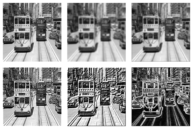
The first image is the original, followed by box filter and Gaussian blur filter. Next is the sharpen filter, then emboss filter and finally Sobel filter that highlights edges.
Thresholding
To actually “see” objects in an image, we need to segment it into foreground and background, and then operate on the foreground segments, trying to locate objects of interest.
This is much easier done when an image is binary, so that each pixel is either fully black or fully white. This conversion from grayscale to black-and-white is called thresholding.
In the simplest case we may consider any pixel above 127 white, and below – black. This is fixed-level thresholding. Of course, in darker environments this thresholding value could be too high and many meaningful details would be lost. So how to pick a threshold value more accurately?
// apply fixed threshold value and binarise the image
GS_API void gs_threshold(struct gs_image img, uint8_t thresh) {
  for (unsigned i = 0; i < img.w * img.h; i++) img.data[i] = (img.data[i] > thresh) ? 255 : 0;
}
One approach would be to calculate the brightness distribution as a histogram. We know that there are 255 unique values of pixels in a grayscale image, so we iterate through all pixels and count how many of them have this or that value. Analysing the resulting histogram could give us some clue about which pixel value would work best as a threshold for the particular image.
A clever way to do this is with Otsu’s method. It automatically determines the optimal threshold by testing every possible value (from 0 to 255). For each value, it splits the image’s pixels into two classes—background and foreground—and calculates their “inter-class variance.” The threshold that maximizes this variance is the one that creates the best separation between the two classes, making it the ideal choice. It works fiarly well on images with good contrast:
// try to find the best threshold to separate "foreground" from "background"
uint8_t gs_otsu_threshold(struct gs_image img) {
  unsigned hist[256] = {0}, wb = 0, wf = 0, threshold = 0;
  // calculate how many pixels of each brightness value we have
  for (unsigned i = 0; i < img.w * img.h; i++) hist[img.data[i]]++;
  float sum = 0, sumB = 0, varMax = -1.0;
  for (unsigned i = 0; i < 256; i++) sum += (float)i * hist[i];
  // try to find the threshold that maximises inter-class variance
  for (unsigned t = 0; t < 256; t++) {
    wb += hist[t];
    if (wb == 0) continue;
    wf = (img.w * img.h) - wb;
    if (wf == 0) break;
    sumB += (float)t * hist[t];
    float mB = (float)sumB / wb;
    float mF = (float)(sum - sumB) / wf;
    float varBetween = (float)wb * (float)wf * (mB - mF) * (mB - mF);
    if (varBetween > varMax) varMax = varBetween, threshold = t;
  }
  return threshold;
}
In real life, however, the lighting conditions are often uneven. In such cases a single global threshold may not work well, and neither of the possible 255 threshold values would give a good result.
To address this, we can use adaptive thresholding. Instead of using a single threshold for the entire image, we compute a local threshold for each pixel based on the average brightness of its neighbouring pixels. This way, we can better handle varying lighting conditions across the image:
gs_for(src, x, y) {
  unsigned sum = 0, count = 0;
  for (int dy = -radius; dy <= (int)radius; dy++) {
    for (int dx = -radius; dx <= (int)radius; dx++) {
      int sy = (int)y + dy, sx = (int)x + dx;
      if (sy >= 0 && sy < (int)src.h && sx >= 0 && sx < (int)src.w) {
        sum += gs_get(src, sx, sy);
        count++;
      }
    }
  }
  int threshold = sum / count - c;
  gs_set(dst, x, y, (gs_get(src, x, y) > threshold) ? 255 : 0);
}
Compare how various thresholding approaches work on the same image:
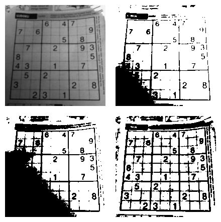
The first image is the original, followed by fixed-level thresholding (80), then Otsu’s method and adaptive thresholding. Notice how adaptive thresholding preserves more details in both bright and dark areas of the image, while Otsu’s method struggles with uneven lighting.
Morphological operations
Due to the way how image sensors work in cameras, images often contain noise.
This means that after thresholding there would be random individual pixels that do not belong to any object, or small holes in objects, or small gaps between object parts. All of this will confuse the object detection algorithms, but morphological operations can help to clean up the binary image.
Two most common operations are erosion and dilation. Erosion removes pixels on object boundaries (shrinking the objects), while dilation adds pixels to their boundaries (expanding the objects).
There is also opening (erosion followed by dilation) and closing (dilation followed by erosion). Opening is useful for removing small objects or noise, while closing is useful for filling small holes in objects.
void gs_erode(struct gs_image dst, struct gs_image src, unsigned radius) {
  gs_for(dst, x, y) {
    uint8_t min_val = 255;
    for (int dy = -radius; dy <= (int)radius; dy++) {
      for (int dx = -radius; dx <= (int)radius; dx++) {
        int sy = (int)y + dy, sx = (int)x + dx;
        if (sy >= 0 && sy < (int)src.h && sx >= 0 && sx < (int)src.w) {
          uint8_t val = gs_get(src, sx, sy);
          if (val < min_val) min_val = val;
        }
      }
    }
    gs_set(dst, x, y, min_val);
  }
}
void gs_dilate(struct gs_image dst, struct gs_image src, unsigned radius) {
  gs_for(dst, x, y) {
    uint8_t max_val = 0;
    for (int dy = -radius; dy <= (int)radius; dy++) {
      for (int dx = -radius; dx <= (int)radius; dx++) {
        int sy = (int)y + dy, sx = (int)x + dx;
        if (sy >= 0 && sy < (int)src.h && sx >= 0 && sx < (int)src.w) {
          uint8_t val = gs_get(src, sx, sy);
          if (val > max_val) max_val = val;
        }
      }
    }
    gs_set(dst, x, y, max_val);
  }
}
Here’s how morphological operations can clean up a rather confusing image with ArUco markers:
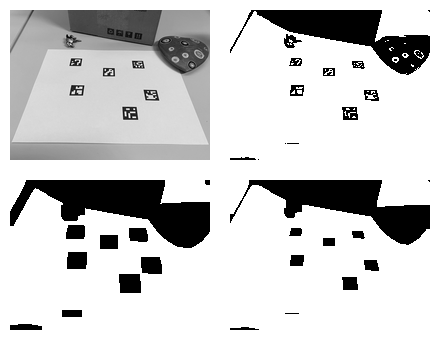
The first image is the original, followed by thresholded image (Otsu). Next we do erosion followed by dilation. Since the markers are black it might sound odd, but since morpological operations work on white pixels we essentially perform closing, but for black pixels. We could also invert the image first, then do opening and invert back.
At the end all markers are shrinked to their original dimensions and all of them are easily detectable by shape and size.
Blobs and contours
Once we have a clean binary image, we can start detecting objects in it. A classic way to do this is by finding connected components (blobs).
A “blob” is a group of connected white pixels (255) that form an object. The simplest way to find blobs is by using a flood-fill algorithm or depth-first search (DFS) to label connected pixels:
void gs_flood_fill(struct gs_image img, unsigned x, unsigned y, uint8_t target, uint8_t replacement) {
  if (x >= img.w || y >= img.h) return;
  if (gs_get(img, x, y) != target || gs_get(img, x, y) == replacement) return;
  gs_set(img, x, y, replacement);
  gs_flood_fill(img, x + 1, y, target, replacement);
  gs_flood_fill(img, x - 1, y, target, replacement);
  gs_flood_fill(img, x, y + 1, target, replacement);
  gs_flood_fill(img, x, y - 1, target, replacement);
}
Of course this would immediately blow up your stack on most real-life images. So an iterative approach using a queue or stack is preferred.
However, it’s still a fairly suboptimal way to find blobs. A more efficient approach is a two-pass algorithm, which scans the image twice: first to assign “provisional” labels and record equivalences between them, followed by the second scan to resolve these equivalences and assign final unique labels to every blob.
It would be nice if we could use the same gs_image type for labels, but in most cases it would require more than 256 labels (especially for temporary provisional labels). So we need a separate array of larger integers to store labels:
typedef uint16_t gs_label; // 64K should be enough, right?

struct gs_blob {
  gs_label label; // what label the blob has?
  unsigned area; // how many white pixels are in a blob?
  struct gs_rect box; // bounding box
  struct gs_point centroid; // center of "mass"
};
unsigned gs_blobs(struct gs_image img, gs_label *labels, struct gs_blob *blobs, unsigned nblobs) { ... }
Before we go futher, let’s talk about connectivity. There are two common types of pixel connectivity: 4-connectivity and 8-connectivity. In 4-connectivity, a pixel is connected to its four direct neighbours (up, down, left, right). In 8-connectivity, a pixel is connected to all eight surrounding pixels (including diagonals). So, in case of 8-connectivity this would be one blob and in case of 4-connectivity - two separate blobs:
......
.#..#.
.##.#.
.###..
......
We will be using 4-connectivity in our implementation, for simplicity. Let’s consider the following image:
.........
.###..#..
.###.##..
.#####..#
.......##
We start scanning it row after row, if a white pixel is found, we check its left and top neighbours:
- If both are black (0), we assign a new label to the pixel, assuming that it could be a new blob.
- If one of them is white, we assign its label to the current pixel, as it is a continuation of the existing known blob.
- If both are white but have different labels, we assign the smallest of the labels to the current pixel and record the equivalence between the two labels in a special data structure (like a union-find).
After this first pass the labels array would look like this:
.........
.111..2..
.111.32..
.11111..4
.......55
Our equivalence table would look like this: 1 <-> 3, 3 <-> 2, 4 <-> 5.
During the second pass we resolve the equivalences and assign final labels to each pixel. The final labels array would look like this:
.........
.111..1..
.111.11..
.11111..4
.......44
During the second pass we can also calculate blob properties, such as area, bounding box and centroid. Largest blob’s area is 14 pixels, bounding box is from (1,1) to (6,3). Centroid is calculated as the average of all pixel coordinates in the blob, in our case for X it would be (3*1+3*2+3*3+4+2*5+2*6)/14, or rounded to 4. Y coordinate would be (4*1+5*2+5*3)/14, or rounded to 2. So the centroid is (4,2), which is not part of the blob “body”, but still is the center of mass.
Such geometric properties already give us plenty of information about blobs. For example, we can filter blobs by area to remove small noise blobs. We can also calculate aspect ratio (width/height) of the bounding box to filter out very tall or very wide blobs. Ratio between blob actual area and bounding box area helps to filter out blobs that are not compact enough. Rectangles tend to have a ratio of 1.0, circles are pi/4 = 0.785, while lines approach to zero.
Another clues could be centroid position, orientation using moments or contour shape. There is a fairly simple method to trace a contour of a blob using the Moore-Neighbor tracing algorithm. It starts from a known border pixel and follows the contour clockwise by checking neighbouring pixels, until it returns to the starting pixel:
struct gs_contour { struct gs_rect box; struct gs_point start; unsigned length; };
void gs_trace_contour(struct gs_image img, struct gs_image visited, struct gs_contour *c) {
  static const int dx[] = {1, 1, 0, -1, -1, -1, 0, 1};
  static const int dy[] = {0, 1, 1, 1, 0, -1, -1, -1};
  c->length = 0;
  c->box = (struct gs_rect){c->start.x, c->start.y, 1, 1};
  struct gs_point p = c->start;
  unsigned dir = 7, seenstart = 0;
  for (;;) {
    if (!visited.data[p.y * visited.w + p.x]) c->length++;
    visited.data[p.y * visited.w + p.x] = 255;
    int ndir = (dir + 1) % 8, found = 0;
    for (int i = 0; i < 8; i++) {
      int d = (ndir + i) % 8, nx = p.x + dx[d], ny = p.y + dy[d];
      if (nx >= 0 && nx < (int)img.w && ny >= 0 && ny < (int)img.h &&
          img.data[ny * img.w + nx] > 128) {
        p = (struct gs_point){nx, ny};
        dir = (d + 6) % 8;
        found = 1;
        break;
      }
    }
    if (!found) break;  // open contour
    c->box.x = GS_MIN(c->box.x, p.x);
    c->box.y = GS_MIN(c->box.y, p.y);
    c->box.w = GS_MAX(c->box.w, p.x - c->box.x + 1);
    c->box.h = GS_MAX(c->box.h, p.y - c->box.y + 1);
    if (p.x == c->start.x && p.y == c->start.y) {
      if (seenstart) break;
      seenstart = 1;
    }
  }
}
This way we can extract contours for each blob and analyse their shapes or compare contour length (perimeter) to the blob area. It is also possible to approximate contours with straight lines using Douglas-Peucker algirithm, which replaces a curve with a series of straight line segments, while preserving the overall shape.
All of this is good if we want to detect simple objects in a static image. But what if we want to detect or track more complex objects, like faces, cars or pedestrians?
Keypoints and descriptors
A keypoint is a specific location in an image that is distinctive and can be reliably detected no matter what scale, rotation or lighting of the object are.
In practice, keypoints are often corners (also known as “features”). One of the most intuitive algorithms to detect features is FAST (Features from Accelerated Segment Test). It works by examining a circle of 16 pixels around a candidate pixel (4 pixels away from it). If at least 9 of contiguous pixels in this r=4px circle around pixel P are all brighter or all darker - then the candidate pixel is considered a corner:
..............
......012.....
.....F...3....
....E.....4...
....D..P..5...
....C.....6...
.....B...7....
......A98.....
..............
As simple as it gets, this approach finds too many features in real-life images. A solution is to keep “score” of each feature and only keep the points with the highest score. The score can be calculated as the sum of absolute differences between the candidate pixel and the contiguous pixels in the circle, or by the minimum difference between central pixel and the pixels on the circle.
  gs_assert(gs_valid(img) && kps && nkps > 0);
  static const int dx[16] = {0, 1, 2, 3, 3, 3, 2, 1, 0, -1, -2, -3, -3, -3, -2, -1};
  static const int dy[16] = {-3, -3, -2, -1, 0, 1, 2, 3, 3, 3, 2, 1, 0, -1, -2, -3};
  unsigned n = 0;
  // first pass: compute score map
  for (unsigned y = 3; y < img.h - 3; y++) {
    for (unsigned x = 3; x < img.w - 3; x++) {
      uint8_t p = img.data[y * img.w + x];
      int run = 0, score = 0;
      for (int i = 0; i < 16 + 9; i++) {
        int idx = (i % 16);
        uint8_t v = img.data[(y + dy[idx]) * img.w + (x + dx[idx])];
        if (v > p + threshold) {
          run = (run > 0) ? run + 1 : 1;
        } else if (v < p - threshold) {
          run = (run < 0) ? run - 1 : -1;
        } else {
          run = 0;
        }
        if (run >= 9 || run <= -9) {
          score = 255;
          for (int j = 0; j < 16; j++) {
            int d = gs_get(img, x + dx[j], y + dy[j]) - p;
            if (d < 0) d = -d;
            if (d < score) score = d;
          }
          break;
        }
      }
      scoremap.data[y * img.w + x] = score;
    }
  }
  // second pass: non-maximum suppression
  for (unsigned y = 3; y < img.h - 3; y++) {
    for (unsigned x = 3; x < img.w - 3; x++) {
      int s = scoremap.data[y * img.w + x], is_max = 1;
      if (s == 0) continue;
      for (int yy = -1; yy <= 1 && is_max; yy++) {
        for (int xx = -1; xx <= 1; xx++) {
          if (xx == 0 && yy == 0) continue;
          if (scoremap.data[(y + yy) * img.w + (x + xx)] > s) {
            is_max = 0;
            break;
          }
        }
      }
      if (is_max && n < nkps) kps[n++] = (struct gs_keypoint){{x, y}, (unsigned)s, 0, {0}};
    }
  }
  return n;
}
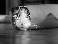
Notice how keypoints are detected on corners and distinctive features of the cat image, such as eyes, nose, whiskers and other “meaningful” corners. But how to use keypoints to detect objects?
This is where ORB enters the stage. ORB builds on top of the same FAST corner detector, it tries to find sharp intensity changes, but also adds two more components: orientation and descriptor.
Once the corners are found, ORB estimates their orientation by calculating image moments in a small patch around each keypoint. This way, each keypoint gets an angle, basically saying which way is “up” for this keypoint.
Then comes the descriptor. A descriptor is a compact representation of the local image patch around the keypoint, designed to be invariant to scale and rotation. ORB uses a modified version of BRIEF (Binary Robust Independent Elementary Features) descriptor, which is a clever way to encode image patch as a small bit string.
It simply compares bit intensities, if one pixel is lighter than another, it sets the corresponding bit to 1, otherwise to 0. By performing multiple such comparisons, we can create a binary string that represents the local image patch.
The descriptor is 256 bit long, and for each of the 256 “samples” we pick two sampling points within the patch area using some pseudo-random lookup table and encode the following bit as 0 or 1 depending on the pixel relative values.
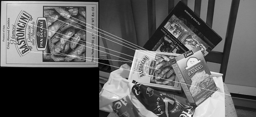
Comparing keypoints becomes trivial, we simply XOR two bitstrings and count the bits.
Since keypoints are agnostic to rotation and lighting conditions, we can use them to detect objects in various scenarios.
One last addition to this algorithm is to resize/scale the image multiple times and detect keypoints at different scales. This way we can detect objects that are closer or further away from the camera, rotated at any angle, or partially occluded.
LBP Cascades
While keypoints and descriptors are great for detecting arbitrary objects, sometimes we need a more specialised approach for specific object types, like faces, vehicles, or hand gestures. This is where cascade classifiers, famously used in the Viola-Jones object detection framework, come into play.
Instead of complex Haar-like features used by Viola and Jones, we can use something simpler: Local Binary Patterns (LBP). LBP is a powerful texture descriptor. For each pixel, it looks at its 8 neighbours. If a neighbour is brighter than the central pixel, we write a ‘1’, otherwise a ‘0’. This gives us an 8-bit number that describes the local texture.
The “cascade” is a series of simple classifiers, or “stages”. Each stage looks at a sub-window of the image and uses a few LBP features to decide if that window could possibly contain the object of interest (e.g., a face).
- If the sub-window fails the test at any stage, it’s immediately rejected. This is very fast.
- Only if a sub-window passes all stages is it classified as a positive detection.
This structure allows the classifier to quickly discard the vast majority of the image, focusing computational power only on promising regions. By sliding this detection window across the entire image (and across multiple scales), we can find objects of a specific, pre-trained class. Grayskull provides a pre-trained frontal face detector that uses this exact technique.
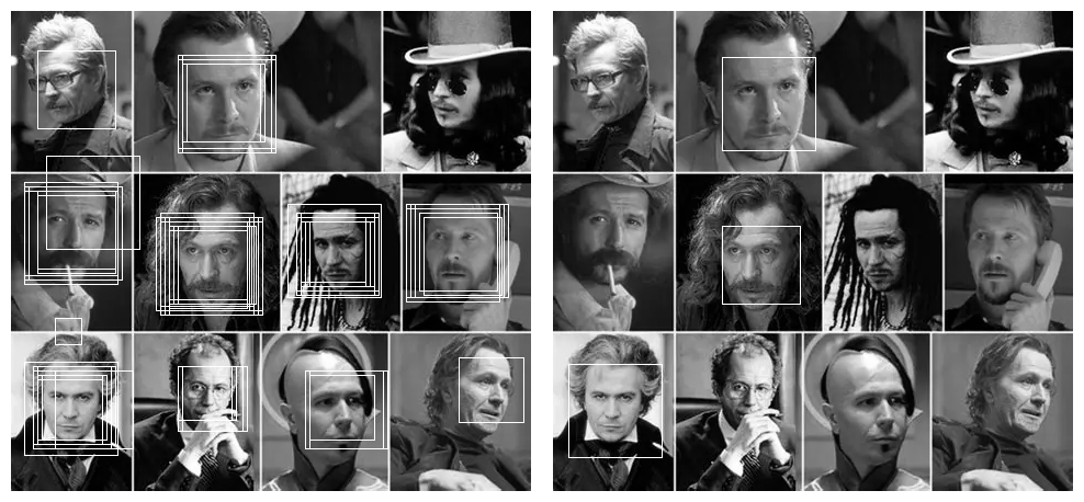
Here you can see the LBP cascade classifier in action, successfully detecting Sir Gary Oldman in all variety of his faces. The picture on the left uses minimum number of neighbours set to 4, while the right one uses 14. This means the left image detects more faces, but also has more false positives, while the right one is more conservative and only detect camera-facing images with no visual obstructions.
Conclusion
We’ve taken a journey from the humble pixel to sophisticated object detection, all using simple C structures and fundamental algorithms. We tried to manipulate pixels, apply filters to enhance images, segment objects using thresholding, and clean them up. We then learned to find and analyze blobs, detect robust keypoints with FAST and ORB, and finally, use LBP cascades for specialized object detection.
This is the core philosophy of Grayskull: to demystify computer vision by providing a minimal, dependency-free, and understandable toolkit. It proves that you don’t always need massive libraries or deep learning frameworks to achieve decent results, especially on resource-constrained systems.
An image is indeed just a rectangle of numbers, and with a bit of algorithmic knowledge, you have the power to make it see. As always, I encourage you to check out the repository, experiment with the code, and maybe even try building your own simple CV project!
I hope you’ve enjoyed this article. You can follow – and contribute to – on Github, Mastodon, Twitter or subscribe via rss.
Oct 26, 2025
See also: Étude in C minor and more.
